
最近參加了機器學習 百日馬拉松的活動,單純記錄下這100天python機器學習中每日覺得最有收穫的地方,如果有想參加這活動的朋友,真心推薦參加!此次機器學習-百日馬拉松的相關代碼放置於:https://github.com/hsuanchi/ML-100-days
相關文章:[百日馬拉松] 機器學習-資料清理https://www.maxlist.xyz/2019/03/03/ml_100days/
目錄
一. 標籤編碼 ( Label Encoding )
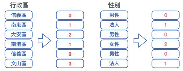
- 類似於流⽔號,依序將新出現的類別依序編上新代碼,已出現的類別編上已使⽤的代碼
- 確實能轉成分數,但缺點是分數的⼤⼩順序沒有意義
|
1 2 3 |
df_temp = pd.DataFrame() for c in df.columns: df_temp[c] = LabelEncoder().fit_transform(df[c]) |
二. 獨熱編碼 ( One Hot Encoding )
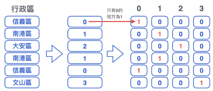
- 為了改良數字⼤⼩沒有意義的問題,將不同的類別分別獨立為⼀欄
- 缺點是需要較⼤的記憶空間與計算時間,且類別數量越多時越嚴重
|
1 |
df_temp = pd.get_dummies(df) |
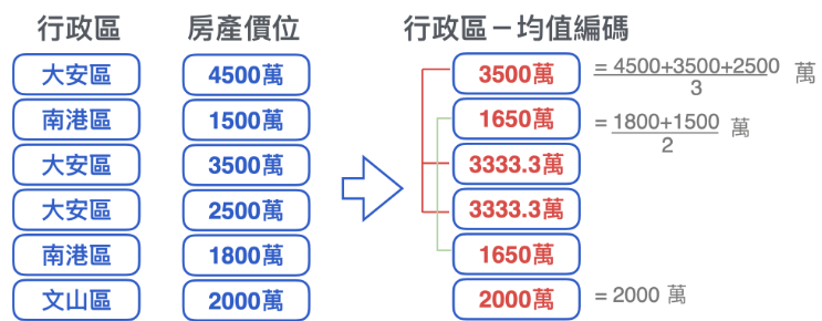
三. 均值編碼 (Mean Encoding)
|
1 2 3 4 5 6 |
for col in object_features: print(col) df_mean = data.groupby([col]['Survived'].mean().reset_index() df_mean.columns = [col, f"{col}_mean"] data = pd.merge(data, df_mean, on=col, how='left') data = data.drop([col], axis=1) |
四. 計數編碼 ( Counting )
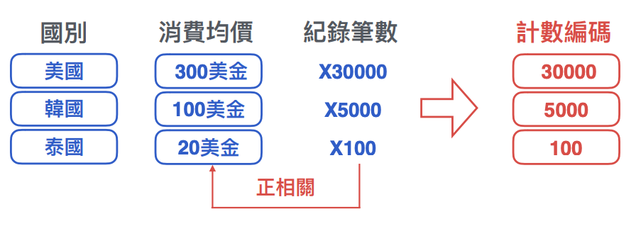
- 如果類別的⽬標均價與類別筆數呈正相關 ( 或負相關 ),也可以將筆數本⾝當成特徵
|
1 2 |
df_count = df.groupby('Cabin')['Name'].agg('size').reset_index()<br>df_count.columns = ['Cabin', 'Cabin_Count']<br>df = pd.merge(df, df_count, on='Cabin', how='left')<br>df.head() df_temp = pd.DataFrame()<br>for col in object_features:<br> df_temp[col] = LabelEncoder().fit_transform(df[col])<br>df_temp['Cabin_Hash'] = df['Cabin'].map(lambda x: hash(x) % 10) |
五. 群聚編碼 (Group by Encoding)
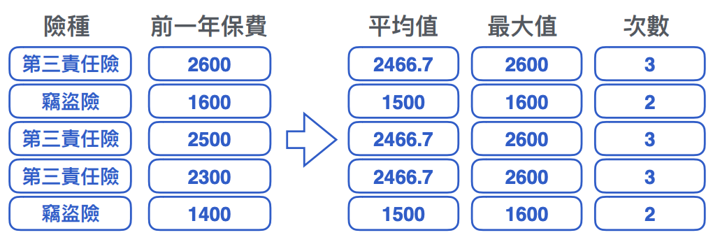
- 數值型特徵對⽂字型特徵最重要的特徵組合⽅式
- 常⾒的有 mean, median, mode, max, min, count 等
|
1 2 3 4 5 6 7 8 |
mean_df = df.groupby(['Embarked'])['Fare'].mean().reset_index() mode_df = df.groupby(['Embarked'])['Fare'].apply(lambda x: x.mode()[0]).reset_index() median_df = df.groupby(['Embarked']['Fare'].median().reset_index() max_df = df.groupby(['Embarked'])['Fare'].max().reset_index() temp = pd.merge(mean_df, mode_df, how='left', on=['Embarked']) temp = pd.merge(temp, median_df, how='left', on=['Embarked']) temp = pd.merge(temp, max_df, how='left', on=['Embarked']) temp.columns = ['Embarked', 'Fare_Mean', 'Fare_Mode', 'Fare_Median', 'Fare_Max'] |
六. 葉編碼(leaf encoding)
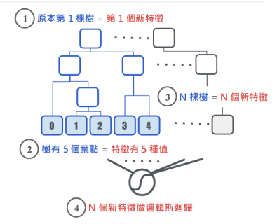
- 將決策樹的葉點當做新特徵
- 再用邏輯回歸合併預測
|
1 2 3 4 5 6 7 8 9 10 11 |
# 隨機森林擬合後 rf = RandomForestClassifier(n_estimators=20, min_samples_split=10, min_samples_leaf=5, max_features=4, max_depth=3, bootstrap=True) 將葉編碼 (*.apply) 結果做獨熱 / 邏輯斯迴歸 onehot = OneHotEncoder() lr = LogisticRegression(solver='lbfgs', max_iter=1000) rf.fit(train_X, train_Y) onehot.fit(rf.apply(train_X)) lr.fit(onehot.transform(rf.apply(val_X)), val_Y) |
七. 特徵雜湊 ( Feature Hash )
- 特徵雜湊是⼀種折衷⽅案
- 將類別由雜湊函數定應到⼀組數字
- 調整雜湊函數對應值的數量
- 在計算空間/時間與鑑別度間取折衷
- 也提⾼了訊息密度, 減少無⽤的標籤
|
1 2 3 4 |
df_temp = pd.DataFrame() for col in object_features: df_temp[col] = LabelEncoder().fit_transform(df[col]) df_temp['Cabin_Hash'] = df['Cabin'].map(lambda x: hash(x) % 10) |
八. 空缺值:
|
1 2 3 |
df_m1 = df.fillna(-1) df_0 = df.fillna(0) df_md = df.fillna(df.median()) |
九. 標準化:
|
1 2 3 |
from sklearn.preprocessing import MinMaxScaler, StandardScaler df_mm = MinMaxScaler().fit_transform(df) df_sc = StandardScaler().fit_transform(df) |
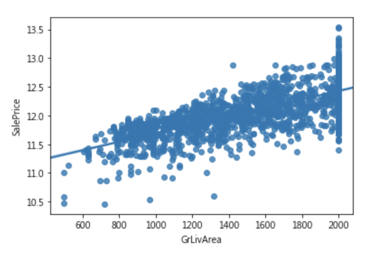
十. 離群值:
|
1 2 3 4 |
#限制離群值在500-2000內 df['GrLivArea'] = df['GrLivArea'].clip(500, 2000) sns.regplot(x = df['GrLivArea'], y=train_Y) plt.show() |
|
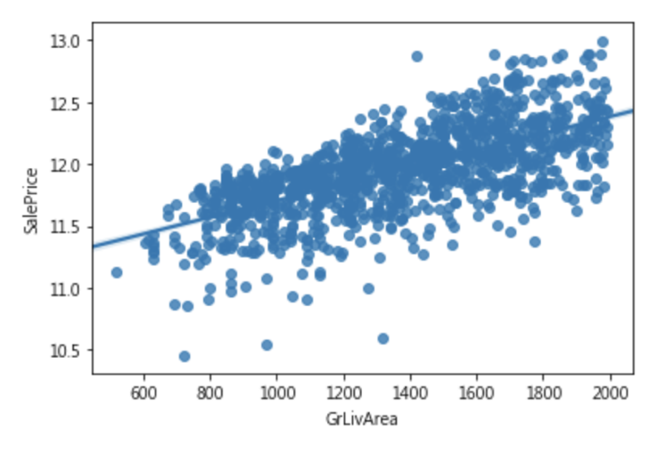
1 2 3 4 5 6 |
#捨棄離群值 keep_indexs = (df['GrLivArea']> 500) & (df['GrLivArea']< 2000) df = df[keep_indexs] train_Y = train_Y[keep_indexs] sns.regplot(x = df['GrLivArea'], y=train_Y) plt.show() |
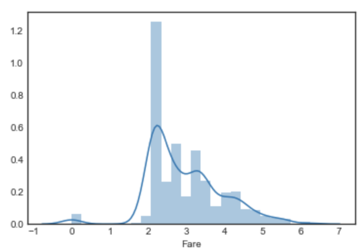
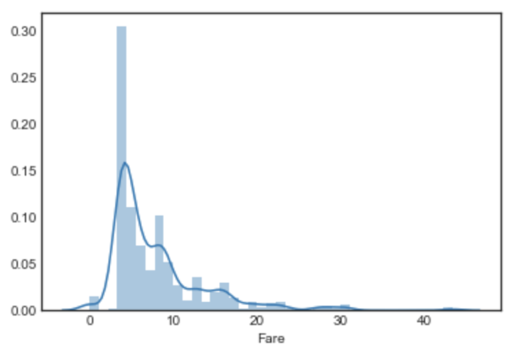
十一. 去偏態:
|
1 2 |
#原始 sns.distplot(df['Fare']) |

|
1 2 3 4 |
# 對數去偏 (log1p) df_fixed['Fare'] = np.log1p(df_fixed['Fare']) sns.distplot(df_fixed['Fare'][:train_num]) plt.show() |
|
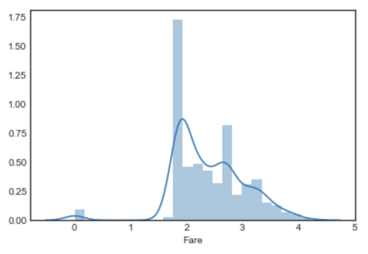
1 2 3 4 5 |
# 分佈去偏(boxcox) from scipy import stats df_fixed['Fare'] = stats.boxcox(df_fixed['Fare']+1)[0] sns.distplot(df_fixed['Fare'][:train_num]) plt.show() |
|
1 2 3 4 |
# ⽅根去偏(sqrt) df_fixed['Fare'] = stats.boxcox(df['Fare']+1, lmbda=0.5) sns.distplot(df_fixed['Fare'][:train_num]) plt.show() |
十二. 特徵工程流程:
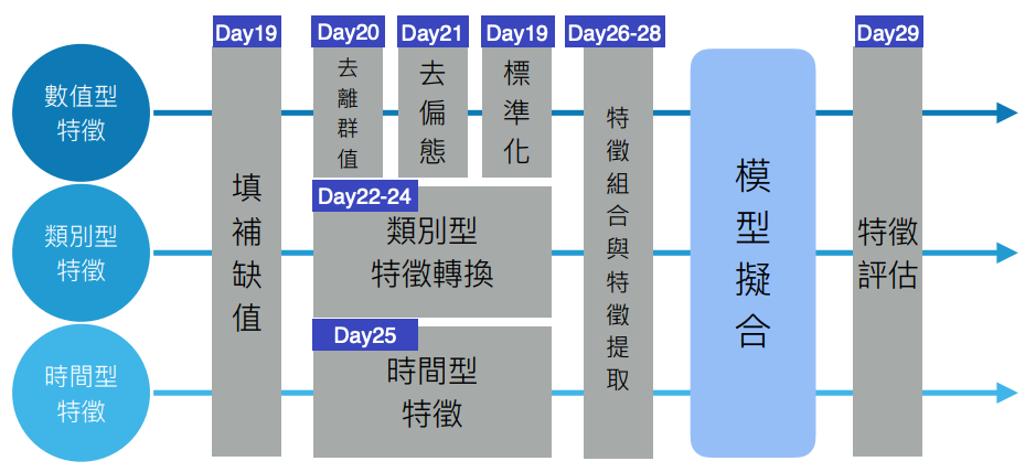
- 讀取資料
- 分解重組與轉換
- train+test=df
- 特徵工程
- Label Encoder
- MinMax Encoder
- 訓練模型與預測
- 提交